Prepared by: Openzeka Teknoloji A.Ş. — Official Embedded Compute Distributor for NVIDIA Türkiye & MEA, and NVIDIA Elite Partner
A Technical Guide on Hardware Architecture, Format and Reliability
Audience: developers serving LLMs, MLOps teams and practitioners Published: October 2026
Table of contents
- 1. Brief Summary
- 2. What Does Quantization Buy You?
- 3. Why Does Quantization Improve Performance?
- 4. GPU Architecture and Quantization Format
- 5. Quantization Formats
- 6. “4-bit = 4-bit” Is Not True
- 7. Why Is NVFP4 Different?
- 8. GPU Architecture × Format Matching
- 9. Ampere: Do Not Confuse INT4 with FP8
- 10. Ada and Hopper: FP8’s Strong Position
- 11. Blackwell: FP8 or NVFP4?
- 12. Mixed-Precision Quantization
- 13. Why Does Calibration Matter?
- 14. How to Choose a Reliable Quantized Checkpoint?
- 15. What Should a Good Model Card Disclose?
- 16. How Should a Benchmark Be Read?
- 17. Case Examples
- 18. PTQ or QAT?
- 19. Quantization Selection Flow
- 20. Common Mistakes
- 1. Moving to 4-bit needlessly when the hardware is enough for the original model
- 2. Crediting the original model’s benchmark to the quantized model
- 3. Saying “4-bit = 4-bit”
- 4. Confusing native hardware acceleration with software support
- 5. Measuring only tokens/s
- 6. Forgetting the KV cache
- 7. Ignoring calibration information
- 8. Trusting only the general benchmark
- 21. Summary Decision Table
- 22. Quick Command Reference
- 23. Evaluating Quantization Quality
- 24. Glossary
- 25. Conclusion
- 26. References
1. Brief Summary
Quantization lets LLM weights — and, where needed, activation/KV cache data — be represented at a lower precision (numeric representation width, i.e. bit width), reducing memory consumption, memory bandwidth demand, and, on suitable hardware, computation cost.
Once seen mostly as “the compromise you reach for when the model does not fit in memory”, it is now the case that formats like FP8 and FP4 are accelerated in hardware on modern GPUs. Many model developers also release official, pre-quantized checkpoints directly.
But quantization by itself does not mean “lower bits = faster”.
The right choice sits at the intersection of four factors:
Workload × Quantization format × GPU architecture × Checkpoint reliability
Three core rules
1. If the model owner ships an official quantized checkpoint, evaluate that first.
That does not automatically make it the highest-quality checkpoint; but in terms of quantization method, format and target runtime it is usually the most reliable starting point.
2. The format must match the GPU architecture.
For example:
- Ampere → INT4/INT8-based methods
- Ada → FP8
- Hopper → FP8
- Blackwell → FP8 / NVFP4 / MXFP4
A format merely “running” without native Tensor Core support does not mean it runs fast.
3. The original model’s benchmark is not the quantized checkpoint’s benchmark.
The BF16 model’s score must not be assumed valid for the same model’s FP8 or FP4 checkpoint.
For a quantized checkpoint, also check:
- the quantization method used,
- the calibration process,
- the benchmark results,
- the runtime,
- the GPU,
- the generation settings
2. What Does Quantization Buy You?
Quantization has three fundamental effects:
- Model weights get smaller
- Memory bandwidth demand drops
- Low-precision Tensor Core computation is accelerated on suitable hardware
How much each matters depends on the workload.
2.1 Memory consumption
In the ideal case, weight memory is roughly:
Parameter count × bytes/parameter
For example:
| Precision (bit width) | Bits | 7B | 70B | 405B |
|---|---|---|---|---|
| BF16 / FP16 | 16 | ~14 GB | ~140 GB | ~810 GB |
| FP8 / INT8 | 8 | ~7 GB | ~70 GB | ~405 GB |
| 4-bit | 4 | ~3.5 GB | ~35 GB | ~202 GB |
These are only ideal weight sizes.
Actual GPU memory is the sum of:
Weights + KV Cache + activations + runtime overhead + quantization metadata
Also remember that in MoE models the total parameter count and the active parameter count differ.
2.2 KV Cache quantization is a separate decision
Weight quantization and KV cache quantization are not the same thing.
For example:
BF16 weights + BF16 KV
BF16 weights + FP8 KV
FP8 weights + FP8 KV
NVFP4 weights + FP8 KV
NVFP4 weights + NVFP4 KV
are entirely different deployment profiles.
With long context and high concurrency, the KV cache can consume a serious amount of GPU memory. For that reason:
Weight quantization
        +
KV Cache quantization
must be considered together.
FP8 KV cache can roughly halve KV memory on a suitable runtime and model architecture; but its effect on attention quality must be verified for the model and implementation at hand.
“It is a significant memory optimization for long context; the effect on model quality must be checked.”
3. Why Does Quantization Improve Performance?
The fundamental purpose of quantization is to reduce memory consumption and data movement by representing model weights at a lower precision, and — where the hardware and kernel support exist — to raise computation throughput.
An LLM’s inference performance can be bounded roughly by two fundamental resources:
- Memory bandwidth: how fast the GPU can move model weights and other data
- Compute throughput: how fast the GPU can perform matrix math with accelerator units like Tensor Cores
Quantization can give an advantage at both points.
3.1 Memory Bandwidth Advantage
When model weights are held at a lower precision, the model gets smaller.
For a model of roughly 70B parameters, for example:
| Precision (bit width) | Approximate weight size |
|---|---|
| FP16 / BF16 | ~140 GB |
| FP8 / INT8 | ~70 GB |
| 4-bit | ~35 GB |
This shrinkage does not only help VRAM capacity. Since inference requires the GPU to move model weights through memory, smaller weights mean less memory traffic.
This can matter especially at low concurrency and in decode-heavy workloads, because when producing a single token, reading the weights from memory can cost a significant amount compared with the computation done on them.
Simplified:
Lower bits → smaller model → less data movement → higher throughput potential in memory-bound workloads
Actual throughput, however, depends on the kernel design, batch size, KV cache, GPU architecture and runtime. A theoretical memory-bandwidth calculation must therefore not be treated as real inference throughput.
3.2 Compute Throughput Advantage
On modern GPUs the advantage of low-precision formats is not only about moving less data.
A GPU’s Tensor Cores perform high-speed matrix math in specific precision formats. If the quantization format used is accelerated at the hardware level, lower precision can also mean higher computation throughput.
For example:
- FP16/BF16 → high-precision Tensor Core math
- FP8 → lower precision and high Tensor Core throughput
- FP4/NVFP4 → very high low-precision Tensor Core throughput on architectures like Blackwell
That is why FP8 or FP4 can bring a significant advantage even when the workload is compute-bound.
In short:
Quantization does not just shrink the model; where the hardware support exists, it also taps the GPU’s higher low-precision compute capacity.
3.3 The Effect of Concurrency and Batch Size
As concurrency and batch size grow, more tokens are processed in parallel on the same model. The GPU’s Tensor Cores are then fed better, and the share of compute throughput in total performance can grow.
So the source of the quantization advantage can vary by workload:
| Workload | Main advantage of quantization |
|---|---|
| Single user / low concurrency | Less memory traffic |
| Medium-high concurrency | Memory + compute advantage |
| Large batch / high throughput | Tensor Core compute throughput rules |
| Compute-bound workload | Low-precision Tensor Core throughput |
| Memory-bound workload | Moving less data |
Quantization, with the right hardware and software support, can both reduce memory bandwidth demand and raise inference throughput by using the GPU’s low-precision compute capacity.
4. GPU Architecture and Quantization Format
A quantization format must not be judged on its own. The performance of the same precision format can differ significantly across GPU architectures.
The fundamental reason is that GPUs support low-precision formats at different levels.
4.1 Why Does Hardware Support Matter?
A format making model weights smaller is no guarantee of high performance by itself.
Consider two different situations:
Situation A — accelerated directly by the hardware
Quantized weights
       ↓
Native GPU Tensor Core
       ↓
High throughput
Situation B — extra conversion / custom kernel required
Quantized weights
       ↓
Dequantization / conversion
       ↓
FP16/BF16 compute
       ↓
Extra cost
In the second case the model may use less VRAM, but the full compute advantage expected may not materialize.
So quantization selection must ask not only:
“How many bits?”
but also:
“How is this format computed on my GPU?”
4.2 General Approach by GPU Generation
| GPU architecture | Notable precision support | General approach |
|---|---|---|
| Ampere | FP16/BF16, INT8/INT4 | INT4/INT8 quantization and optimized kernels are strong choices |
| Ada Lovelace | FP16/BF16, FP8 | FP8 and low-bit quantization can be evaluated |
| Hopper | FP16/BF16, FP8 | FP8 is a strong native acceleration option |
| Blackwell | FP16/BF16, FP8, FP4/NVFP4 | FP8 and especially NVFP4 are significant options |
The point here is not to say “a new format will not run on an older GPU”. Software/runtime support may allow different formats to be used. But native Tensor Core support can make a decisive difference in performance.
4.3 FP8: The Balanced Choice Between Memory and Compute
On architectures like Hopper and Blackwell in particular, FP8 combines two important advantages:
- Lower model memory than FP16/BF16
- Hardware-accelerated high Tensor Core throughput
FP8 is therefore not just a format for squeezing the model into VRAM.
Especially in high-concurrency, throughput-focused inference systems:
Lower memory footprint + higher low-precision compute throughput
can be had together.
One of FP8’s important advantages over 4-bit formats is its higher numeric precision. When preserving quality is critical and the model suits FP8 well, it can be a strong preference.
4.4 FP4 / NVFP4: The Hardware Advantage on Blackwell
With the Blackwell architecture, FP4-class formats have become more important.
NVFP4 in particular must not be judged merely as a “4-bit model”. The format’s purpose is to combine the memory advantage of narrow bit widths with Blackwell’s low-precision Tensor Core support.
NVFP4 can therefore help in two directions:
The memory side
FP16 → FP8 → FP4
 ↓       ↓      ↓
Less model memory
Less data movement
The compute side
FP16/BF16
    ↓
FP8
    ↓
FP4 / NVFP4
    ↓
Blackwell low-precision Tensor Core throughput
So when NVFP4 is on the table on Blackwell, it is not enough to say:
“The model uses less VRAM because it is 4-bit.”
The point that matters is:
NVFP4 can bring an advantage in both memory-bound and compute-bound workloads by combining low memory use with Blackwell’s native low-precision compute capacity.
4.5 The Basic Rule of Quantization Selection
When choosing a quantization format, four factors must be weighed together:
1. Model quality
How much of the model’s accuracy, perplexity and task-level performance survives quantization?
2. Memory footprint
What load do the model and the KV cache put on GPU memory?
3. Hardware acceleration
Does the GPU support this precision format natively through Tensor Cores or another dedicated accelerator?
4. Runtime / kernel support
How efficiently does vLLM, SGLang, TensorRT-LLM, llama.cpp or whatever inference stack you run execute this format?
The format with the lowest bit count is therefore not automatically the fastest.
The right choice:
is made by weighing model quality + memory footprint + native hardware acceleration + runtime/kernel support together.
5. Quantization Formats
| Format / method | Typical use | Main advantage |
|---|---|---|
| GGUF | llama.cpp / CPU+GPU | Flexibility, broad hardware support |
| GPTQ | NVIDIA inference | Widespread weight-only quantization |
| AWQ | NVIDIA inference | Activation-aware weight quantization |
| EXL2 | NVIDIA / ExLlama | Quality-speed trade-off with variable bpw |
| INT8 / SmoothQuant | Inference | Strong option when moving to low precision |
| NF4 / bitsandbytes | QLoRA / fine-tuning | Training / fine-tuning ecosystem |
| FP8 | Ada / Hopper / Blackwell | Native low-precision acceleration |
| NVFP4 | Blackwell | Very low memory + native FP4 acceleration |
| MXFP4 | Blackwell and supporting platforms | Open MX standard, aimed at portability |
6. “4-bit = 4-bit” Is Not True
Two quantization methods with the same nominal bit width may give different quality or performance.
For example:
INT4
AWQ
GPTQ
NF4
MXFP4
NVFP4
all fall in the “4-bit” class, yet these can differ:
- number representation,
- scaling,
- block size,
- calibration,
- weight-only / weight+activation approach,
- kernel,
- hardware acceleration
Hence:
“4-bit model”
is not a sufficient technical definition on its own.
A more accurate definition:
“NVFP4, a Blackwell-optimized 4-bit floating-point format using 16-element micro-block FP8 scaling”
should include the format’s details like this.
7. Why Is NVFP4 Different?
NVIDIA NVFP4 is the 4-bit floating-point format designed for Blackwell.
Its basic approach is:
FP4 values
    +
FP8 micro-scale
    +
FP32 tensor-level scale
In NVFP4, FP4 values are scaled with an FP8 scale over 16-element micro-blocks. A tensor-level FP32 scale is used as well.
This approach aims to reduce quantization error compared with a plain FP4 representation.
According to data published by NVIDIA, NVFP4 can give a model footprint about 1.8× smaller than FP8 and about 3.5× smaller than FP16; the actual checkpoint size depends on the metadata and the mixed-precision recipe used.
So:
NVFP4 = not just “4 bits”.
The real difference is the combination:
4-bit representation + fine-grained scaling + hardware acceleration
8. GPU Architecture × Format Matching
This is one of the most important decision points.
| GPU architecture | Preferred options | Note |
|---|---|---|
| Pascal | GGUF Q4/Q5/Q6 | No modern FP8/FP4 Tensor Core features |
| Turing | INT8 / INT4-based methods | No native FP8 Tensor Core support |
| Ampere | INT4 / INT8, AWQ/GPTQ | A100 supports native INT4/INT8 Tensor Cores |
| Ada | FP8, INT4 | Native FP8 Tensor Core support |
| Hopper | FP8 | FP8 + Transformer Engine is a strong choice |
| Blackwell | NVFP4 / FP8 / MXFP4 | Native FP4 and FP8 acceleration |
“Preferred” here does not mean the format is automatically best for every model.
Model, runtime and workload must still be evaluated.
9. Ampere: Do Not Confuse INT4 with FP8
Ampere matters especially for this reason:
A100 / RTX 30
        ↓
Native INT4 / INT8 Tensor Core
        ↓
AWQ / GPTQ / Marlin-style INT4 deployments
The A100 has INT4 Tensor Core support.
FP8, by contrast, is a precision that came into its own with Hopper and is also supported on Ada.
So on Ampere one must not assume:
“There is an FP8 file, so it must be faster.”
A runtime may execute an FP8 checkpoint in some form; but native hardware acceleration and software-level support are not the same thing.
For 4-bit deployments on Ampere:
AWQ/GPTQ + a suitable optimized kernel
is the more sensible starting point in most cases.
10. Ada and Hopper: FP8’s Strong Position
Ada Lovelace offers FP8 Tensor Core acceleration.
Hopper takes FP8 further with the Transformer Engine.
So:
Ada
 → FP8 is a serious option

Hopper
 → FP8 is a strong default for production inference
But one must not claim:
“FP8 is always 2× faster than FP16.”
Numbers like 2× can express theoretical or peak advantages under specific kernel/throughput conditions. Real LLM throughput varies with model architecture, batch, sequence length and runtime.
11. Blackwell: FP8 or NVFP4?
On Blackwell the central question is no longer just:
“Can I reduce the model to 4-bit?”
The better question is:
“For this model, which suits better in quality, memory and throughput: FP8 or FP4?”
FP8
Advantages:
- higher numeric precision
- generally lower quantization error
- native Blackwell acceleration
- a strong option in quality-critical workloads
NVFP4
Advantages:
- lower weight footprint
- lower memory traffic
- native Blackwell FP4 acceleration
- the advantage of fitting larger models into smaller GPU clusters
Practical approach
FP8
 ↓
Benchmark
 ↓
NVFP4
 ↓
Benchmark
 ↓
Compare quality + latency + throughput + VRAM
The outcome:
Quality difference acceptable
        → NVFP4

Quality critical
        → FP8
This decision must be made model by model.
12. Mixed-Precision Quantization
Modern quantized checkpoints often do not store all weights in the same format.
For example, a recipe like this may be used:
MLP                 → NVFP4
Attention           → FP8
lm_head             → NVFP4 / higher precision
critical layers     → higher precision
The basic rationale is:
Not every layer is equally sensitive to quantization error.
A good quantization pipeline can therefore proceed like this:
Model
  ↓
Calibration
  ↓
Layer sensitivity analysis
  ↓
Mixed-precision recipe
  ↓
Quantization
  ↓
Benchmark
So saying only:
“The model is 4-bit.”
is not enough. What really matters is:
- which layers were quantized?
- which precision was used?
- what is the block size?
- how was scaling done?
- what is the calibration dataset?
- what is the calibration algorithm?
13. Why Does Calibration Matter?
During PTQ (Post-Training Quantization), the calibration dataset should represent the model’s real usage distribution.
For example, choices like these make more sense:
General chat model
    → general text calibration

Coding model
    → coding-weighted calibration

Agent model
    → tool-use / instruction / reasoning calibration
The calibration process can influence where and how quantization error arises.
Hence:
Same model + same 4-bit format ≠ same quality
14. How to Choose a Reliable Quantized Checkpoint?
When choosing a quantized model, the reliability of the source is critical.
Preference order
1. The model owner’s official checkpoint
This is the best starting point.
2. The checkpoint released by the hardware / inference vendor
For example, NVIDIA Model Optimizer-based checkpoints whose benchmark and calibration details are given openly.
3. Quants prepared by the framework / inference community
They can work well; but the metadata and benchmark quality must be checked separately.
4. Community-produced quantization
Quantization files prepared by the community must not be used in production without verifying their source and production process.
The risk here is not only poor quantization quality. A quantized model file must not be considered reliable without verifying:
- who produced it,
- which base model it was derived from,
- with which quantization method and tools it was created,
- which calibration data was used,
- whether the integrity of the model file is preserved,
- whether it is compatible with the runtime and kernels in use
Especially in production systems, models and quantization artifacts of unknown origin become a supply-chain risk. Since model weights and their related files are the fundamental inputs of the inference pipeline that runs them, a reliability decision must not be made from a benchmark score alone.
Known publishers — a starting list
The accounts below are starting points that stand out for their production process and model card transparency. A publisher’s name is not a quality guarantee; it indicates where to begin the search:
| Publisher | Type | Typical formats | Link(s) |
|---|---|---|---|
| NVIDIA (Model Optimizer) | Hardware / production vendor | NVFP4, FP8 (mixed recipe) | HF nvidia · TensorRT-Model-Optimizer |
| RadixArk | SGLang ecosystem | NVFP4, blockwise FP8, MLX 4-bit, DSpark draft | HF RadixArk · cookbook.sglang.ai |
| Inferact | vLLM ecosystem | NVFP4, MXFP4, W4A4, EAGLE3 / DSpark draft | HF Inferact · inferact.ai |
| Red Hat AI | Inference provider | FP8, INT4 (AWQ/GPTQ) | HF RedHatAI |
| Intel | Hardware / runtime vendor | INT8 / INT4 | HF OpenVINO · HF Intel · neural-compressor · openvino |
| ggml-org | Format ecosystem (llama.cpp) | GGUF | HF ggml-org |
| ISTA-DASLab | University research lab — source of GPTQ, SparseGPT, AQLM, QuIP# | GPTQ / MatGPTQ, NVFP4 (MoESQ), GGUF (GSQ-RCO), 2-bit (AQLM / QuIP#) | HF ISTA-DASLab · github.com/IST-DASLab |
LM Studio (lmstudio-community) |
Official model pool of a local inference runtime | GGUF, MLX (4/6/8-bit) | HF lmstudio-community · lmstudio.ai |
| bartowski | Well-known community publisher | GGUF, EXL2 | HF bartowski |
| unsloth | Training + quant ecosystem | 4-bit dynamic quant, GGUF | HF unsloth |
Three rules:
- The order does not change: the model owner’s official quant → hardware / inference vendor → known publisher → your own quant (same as the preference order above).
- The checklist is fixed: however well-known the publisher, nothing enters production without verifying the §15 model card list.
- The list ages: this is a snapshot starting list; confirm each publisher’s current activity and card transparency every time.
Note: The same model may be published by different publishers (e.g.
Qwen3.8-27B-NVFP4exists at NVIDIA, RadixArk and Inferact alike). In that case, comparing publishers must be done with the quality framework in §23. RadixArk and Inferact publish not only quants but also speculative decoding drafts (DSpark / EAGLE3).
15. What Should a Good Model Card Disclose?
A good quantized checkpoint should give the following information as fully as possible. Not all of these carry the same weight, though; start the review with these three tiers.
Critical — the basics that must be verified
Note: What separates two quants is not the nominal bit count but the method + scaling + calibration + recipe (§6, §13). The measured summary of that difference is “a benchmark comparison against the original model” — the most valuable item on the list, and meaningless unless given with its conditions (§16).
- Base model
- Producer / publisher identity
- Quantization method (with weight/activation precision stated)
- Benchmark comparison against the original model (with its conditions: the only measurable evidence of the quality gap between two quants — §16)
Decisive — these settle what is left in doubt
Quantization technical details:
- Calibration dataset + algorithm + sample count (for QAT models, the training / post-training recipe and the quantization simulation instead — see §17.4)
- Weight precision
- Activation precision
- KV cache precision (required only if the benchmark or the recommended deployment was run with a specific KV precision — it is not a checkpoint property in itself but a deployment decision: §2.2)
- Mixed-precision recipe
- Block / group size
Benchmark conditions:
- Evaluation datasets
- Generation settings
- Context length
- GPU + runtime tested
Compatibility / scale:
- Supported GPU architectures
- Tensor parallelism
Supporting — they do not determine technical quality, but their absence causes practical trouble
- Quantization library + version
- File integrity (commit hash / checksum) + release date
- License
The more of this information is missing, the harder it becomes to evaluate a quantized checkpoint independently.
16. How Should a Benchmark Be Read?
When judging a quantized model’s benchmark, the score alone must not be trusted.
For example:
BF16     → 88.92
NVFP4    → 88.01
means little on its own.
These must also be the same:
- benchmark version
- prompt format
- system prompt
- temperature
- top_p
- max_new_tokens
- context length
- reasoning mode
- tool configuration
Otherwise two benchmarks cannot be compared directly.
The most reliable approach is:
BF16 baseline
      ↓
same benchmark
      ↓
same generation settings
      ↓
same runtime
      ↓
quantized model
      ↓
same benchmark
17. Case Examples
The cases represent four basic scenarios, by where the quantized form originates:
- Double release — original BF16; the vendor also ships its own official FP8.
- Direct low-bit release — the original model is released already quantized.
- Third-party quant — the hardware / inference vendor quantizes a model released as BF16.
- 4-bit through QAT — quantization enters the training stage.
These scenarios map to the preference order in §14: 1 and 2 → the model owner’s official checkpoint, 3 → the hardware / inference vendor’s checkpoint, 4 → the model owner (production with QAT).
17.1 Scenario 1 — Original BF16 + Official FP8: Qwen3.8-27B
Qwen/Qwen3.8-27B is a 27B-parameter model.
Alongside it, Qwen also released the
Qwen/Qwen3.8-27B-FP8
checkpoint.
The FP8 checkpoint uses:
- fine-grained FP8
- block size 128
- BF16 + FP8 tensor layout
The Qwen model card states that performance metrics are close to the original model.
Lesson:
Comparing the official FP8 deployment checkpoint against the BF16 baseline within the same model family is a strong start for evaluating quantization.
17.2 Scenario 2 — Direct FP8 Release: GLM-5.3
zai-org/GLM-5.3 is a model in the 753B class and is labeled FP8 in its model repository, alongside BF16, F8_E4M3 and F32 tensor types.
What matters here:
Quantization is no longer only something the community applies afterward.
Model vendors can release low-precision checkpoints directly.
Lesson:
The precision a model is released in becomes part of the deployment architecture.
17.3 Scenario 3 — Third-Party Quant (NVIDIA): Qwen3.8-27B-NVFP4
nvidia/Qwen3.8-27B-NVFP4 is a deployment checkpoint prepared with NVIDIA Model Optimizer.
Its model card states these details explicitly:
- Model Optimizer v0.48.0
- mixed NVFP4/FP8
- NVFP4 → MLP +
lm_head - FP8 → self-attention + linear-attention
- 2.048 calibration samples
- Local-Hessian calibration
- Nemotron-Post-Training-Dataset-v3
- vLLM
- Grace Blackwell GB300
The BF16 and NVFP4 results were also compared on the same benchmark set.
| Benchmark | BF16 | NVFP4 |
|---|---|---|
| GPQA Diamond | 88.92 | 88.01 |
| Terminal-Bench | 75.56 | 74.02 |
| AA-LCR | 72.63 | 73.38 |
| MMMU-Pro | 75.14 | 74.86 |
| SciCode | 47.93 | 48.41 |
| IFBench | 80.07 | 78.93 |
The real lesson matters more than the individual scores:
The quantization recipe + calibration + evaluation methodology are documented openly.
The checkpoint can therefore be examined and reproduced independently.
17.4 Scenario 4 — 4-Bit with QAT: Kimi K3
moonshotai/Kimi-K3 uses:
- 2.8T total parameters
- 104B activated parameters
- 1M context
- MXFP4 weights
- MXFP8 activations
- Quantization-Aware Training (from the SFT stage on)
The inference runtimes the card suggests: vLLM, SGLang and TokenSpeed.
The point that matters:
The model vendor produces the model with quantization-aware training from the SFT stage on, rather than applying quantization afterward, and releases it as MXFP4 / MXFP8. Here quantization is not a “compression step” applied after training; it is a design decision in the model’s path to release.
This example changes several assumptions at once:
1. The assumption “original = BF16, quantized = derivative” no longer holds.
This model’s official release is already 4-bit. There is no “going back to BF16 to recover quality”; the reference checkpoint itself is quantized.
2. Quantization is no longer the last resort; in some models it is the only official form.
This is the strongest example of the “is there an official FP8/FP4 release?” step in the §19 selection flow: the model’s produced quantized form is the model itself.
3. The subject is not only weight quantization.
Taken together, MXFP4 weights + MXFP8 activations is weight+activation (full-tensor) quantization; the extreme example of the weight-only / weight+activation distinction in §6, different from AWQ/GPTQ’s weight-only approach.
4. MXFP4 is the open OCP standard.
It is an example of the portability goal mentioned in §5: an open format family that does not bind you to a single vendor. Moonshot AI’s rationale is exactly this; the card states the MXFP4 / MXFP8 choice was made for “broad hardware compatibility”.
5. Quality validation is read in reverse.
The question is not “how much did 4-bit lose?” but “is the 4-bit operating condition the vendor trained sufficient for my workload?” The answer comes from the model card benchmark read as in §16 and from your own production workload test.
Lesson:
PTQ and QAT are not the same thing.
PTQ:
BF16 model
   ↓
training completed
   ↓
quantization
QAT:
Quantized operating conditions
        ↓
part of the training / post-training process
        ↓
quantized model
Two more lessons follow:
Low bits are not always a “compromise”. In QAT, 4-bit is the target operating condition; quality is optimized for it. The “low bits = accepted loss” perception does not hold for this model class.
The model card checklist (§15) reads differently for QAT models. Instead of a “calibration dataset”, look for the training/post-training recipe and the quantization simulation used in training; the calibration flow in §13 is specific to PTQ.
18. PTQ or QAT?
| Property | PTQ | QAT |
|---|---|---|
| Can be applied after training | Yes | No / needs training |
| Cost | Lower | Higher |
| Fast for deployment | Yes | Longer process |
| Calibration needed | Usually yes | Depends on the recipe |
| Very low precision | Harder | Can be more advantageous |
| Optimizing model quality | Limited | Stronger |
| Practical for an existing model | Very suitable | More costly |
For production deployment, PTQ is the more practical starting point for most users.
But for very low precision or frontier model deployment, QAT can become an important option.
19. Quantization Selection Flow
The practical decision process should look like this:
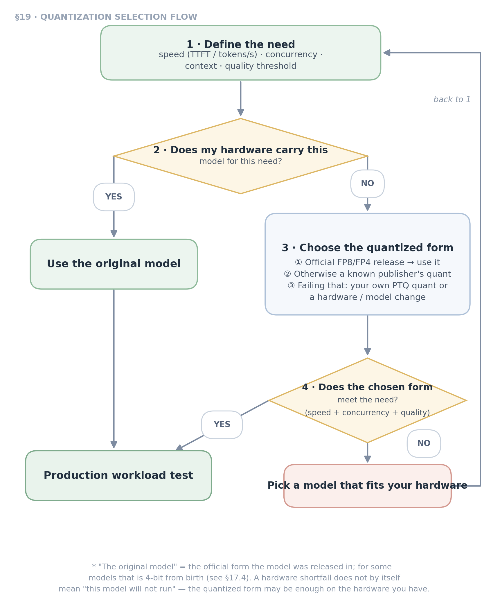
- Define the need: required speed (TTFT / tokens/s), concurrency, context, quality threshold.
- Does my hardware carry this model for this need?
- Yes → use the original model → production workload test.
- No → go to step 3.
- Choose the quantized form:
- If the model has an official FP8/FP4 release → use it.
- Otherwise use a known publisher’s quant (NVIDIA, known framework / community publishers) (see §14).
- If there is none → your own quant (PTQ) or a hardware / model change.
- Does the chosen form deliver what the need asks? (speed + concurrency + quality)
- Yes → production workload test.
- No → pick a model that fits your hardware and start again from step 1.
Note: “Original model” = the official form the model was released in; for some models that is 4-bit from birth (see §17.4).
The basic principle:
A hardware shortfall does not by itself mean “this model will not run”. The model’s quantized form may give the required speed and concurrency on the hardware you have; the goal is not to pick the lowest bits, but to meet the need at a precision the hardware is strong at.
If high throughput or capacity is the target, though, lower precision may be the better economic choice.
20. Common Mistakes
1. Moving to 4-bit needlessly when the hardware is enough for the original model
Lower precision is not always better. If the hardware is enough for the original model — speed, concurrency etc. — there is no reason to pay for quantization (see §19).
2. Crediting the original model’s benchmark to the quantized model
A BF16 result:
is the result of the BF16 checkpoint.
The quantized checkpoint must be verified separately.
3. Saying “4-bit = 4-bit”
AWQ, GPTQ, NF4, MXFP4 and NVFP4 are not the same thing.
4. Confusing native hardware acceleration with software support
A runtime accepting a format does not mean the GPU accelerates that format natively.
5. Measuring only tokens/s
Higher throughput does not mean a better deployment.
TTFT, ITL, latency and concurrency must be measured too.
6. Forgetting the KV cache
Especially in long context, KV cache precision matters as much as weight quantization.
7. Ignoring calibration information
Different calibration recipes of the same format can give different results.
8. Trusting only the general benchmark
If the model’s real use is coding, test coding; if it is an agent, test agentic use; if it is RAG, test long-context retrieval performance.
21. Summary Decision Table
| Scenario | Starting preference |
|---|---|
| Quality critical | BF16 / FP8 |
| Ada | Always evaluate FP8 |
| Hopper production serving | FP8 + a suitable KV cache precision |
| Ampere 4-bit | AWQ/GPTQ + optimized INT4 kernel |
| Blackwell, maximum capacity / throughput | Evaluate NVFP4 |
| Blackwell, quality first | FP8 |
| Multi-vendor deployment | MXFP4 / supported common formats |
| Long context | Weight quantization + KV cache precision together |
| Fine-tuning / QLoRA | NF4 / a suitable training precision |
| Critical production deployment | Official checkpoint + your own workload benchmark |
Note: Set up the hardware × need equation first (see §19): if your hardware carries the model for your need, use the original model; if not, look at the quantized forms.
22. Quick Command Reference
FP8
vllm serve <model> \
  --quantization fp8 \
  --kv-cache-dtype fp8
NVIDIA NVFP4
vllm serve <model-nvfp4> \
  --kv-cache-dtype fp8_e4m3
AWQ / GPTQ
vllm serve <model-awq-or-gptq>
GGUF
llama-server \
  -m model-Q4_K_M.gguf \
  -ngl 99
Comparing quantizations
BF16 baseline
        ↓
FP8
        ↓
NVFP4 / INT4
        ↓
same benchmark
        ↓
same production workload
23. Evaluating Quantization Quality
No single universal threshold should be used.
For example, a general rule like:
“If MMLU drops more than 1%, the quantization has failed.”
is not true.
A 1% loss can be acceptable in some workloads, while in some critical coding or reasoning applications even a very small drop can matter.
The more accurate approach is to weigh these together:
Quality loss
      ×
Business impact
      ×
Performance gain
      ×
Memory saving
For example, with a result like:
FP8
Quality = 100
VRAM = 100
Speed = 1.0

NVFP4
Quality = 99.2
VRAM = 55
Speed = 1.7
NVFP4 may be the more sensible choice.
But if the result is:
Quality = 95
FP8 may be preferred for the same deployment.
The right threshold therefore comes from:
the minimum quality the workload can accept + the performance required + the VRAM available
24. Glossary
BF16 / FP16 Generally the high-precision reference operating formats.
FP8 An 8-bit floating-point format family. It has variants such as E4M3 and E5M2.
NVFP4 The 4-bit floating-point format designed for NVIDIA Blackwell. It uses fine-grained scaling.
MXFP4 The 4-bit floating-point format of the OCP Microscaling format family.
MXFP8 The 8-bit floating-point format of the OCP Microscaling format family. It is preferred for data like activations that need higher numeric precision; for example the MXFP4 weights + MXFP8 activations combination (see §17.4).
AWQ Activation-aware Weight Quantization. Common especially in weight-only INT4 deployments.
GPTQ A post-training weight quantization method.
EXL2 The variable bits-per-weight approach used in the ExLlama ecosystem.
GGUF The model file format used in the llama.cpp ecosystem.
KV cache The cache that stores the Key/Value representation of previous tokens during attention.
PTQ Post-Training Quantization. Applying quantization after training is complete.
QAT Quantization-Aware Training. Incorporating the effects of quantization into the model during training.
Calibration The measurement process on representative data to determine the quantization parameters.
Block size / group size Determines the granularity at which quantization scaling or parameter grouping is applied.
Perplexity One of the fundamental metrics measuring a language model’s prediction performance.
Precision The representation form that states how many bits numeric values (weights, activations, KV cache) are expressed in: “higher precision” = more bits. It is also called hassasiyet in Turkish; but it must not be confused with the model’s accuracy. Lower precision uses fewer bits; it does not automatically mean a more wrong model.
MMLU / GSM8K / GPQA Benchmarks used to measure different capability areas.
25. Conclusion
Quantization must neither be dismissed nor judged as “always faster”.
In modern LLM deployment, quantization is:
a fundamental engineering tool that optimizes between memory capacity, memory bandwidth, Tensor Core throughput and deployment cost.
The right choice cannot be made by looking at the bit count alone.
These four questions must be asked together:
1. At which precision was the model released?

2. Which precision does the GPU accelerate natively?

3. How was the quantization produced, with which calibration recipe?

4. What do quality and performance look like in my real workload?
Their result selects the ideal deployment:
the lowest-cost precision that meets the need, is efficiently accelerated by the GPU, and whose quality loss has been measured.
So the most correct approach to quantization is:
“Pick the lowest bit count.”
No — it must be:
“Keeping the quality my workload requires, pick the precision the hardware is strong at and verify it on a real deployment.”
26. References
- Z.ai — GLM-5.3 Model Card
- Qwen — Qwen3.8-27B Model Card
- Qwen — Qwen3.8-27B-FP8 Model Card
- NVIDIA — Qwen3.8-27B-NVFP4 Model Card
- NVIDIA Model Optimizer — Local-Hessian Quantization
- NVIDIA — Introducing NVFP4 for Efficient and Accurate Low-Precision Inference
- NVIDIA — Hopper Architecture
- NVIDIA — Ada Lovelace Architecture
- NVIDIA — A100 Architecture / Specifications
- NVIDIA TensorRT-LLM — Quantization Hardware Support
- Moonshot AI — Kimi K3 Model Card
- OCP Microscaling Formats — MXFP4 / MXFP8